Supervised Learning with scikit-learn - Part 3
Chapter 3 - How good is your model?
Having trained models, now you will learn how to evaluate them. In this chapter, you will be introduced to several metrics along with a visualization technique for analyzing classification model performance using scikit-learn. You will also learn how to optimize classification and regression models through the use of hyperparameter tuning.
import pandas as pd
import numpy as np
import warnings

pd.set_option('display.expand_frame_repr', False)

warnings.filterwarnings("ignore", category=DeprecationWarning)
warnings.filterwarnings("ignore", category=FutureWarning)
How good is your model?
Classification metrics
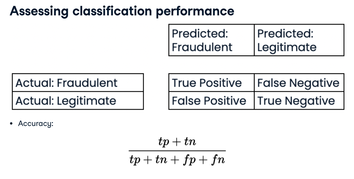
- Measuring model performance with accuracy:
- Fraction of correctly classified samples
- Not always a useful metric
Class imbalance
Classi,cation for predicting fraudulent bank transactions
- 99% of transactions are legitimate; 1% are fraudulent
Could build a classi,er that predicts NONE of the transactions are fraudulent
- 99% accurate!
- But terrible at actually predicting fraudulent transactions
- Fails at its original purpose
Class imbalance: Uneven frequency of classes
- Need a different way to assess performance
churn_df = pd.read_csv('./datasets/telecom_churn_clean.csv',index_col=0)
display(churn_df.head())
display(churn_df.info())

X = churn_df.drop(['churn'], axis=1).values
y = churn_df["churn"].values
print(X.shape, y.shape)
from sklearn.model_selection import train_test_split
from sklearn.neighbors import KNeighborsClassifier
from sklearn.metrics import classification_report, confusion_matrix


knn = KNeighborsClassifier(n_neighbors=7)
X_train, X_test, y_train, y_test = train_test_split(X, y, test_size=0.4, random_state=42)
print(X_train.shape, y_train.shape)

knn.fit(X_train, y_train)
y_pred = knn.predict(X_test)

print(confusion_matrix(y_test, y_pred))
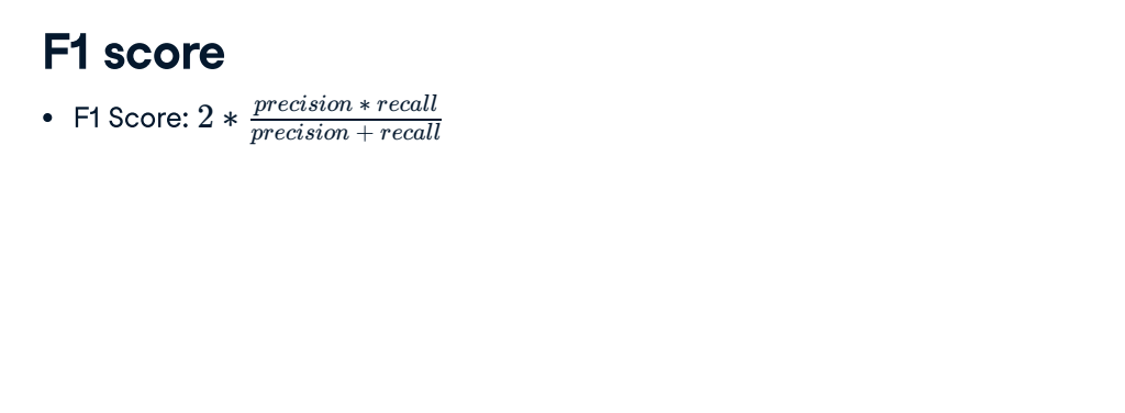
print(classification_report(y_test, y_pred))
Deciding on a primary metric
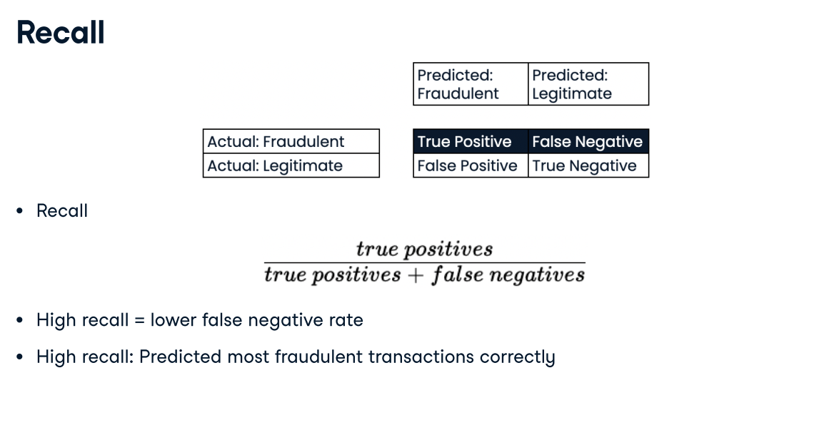
Deciding on a primary metric As you have seen, several metrics can be useful to evaluate the performance of classification models, including accuracy, precision, recall, and F1-score.
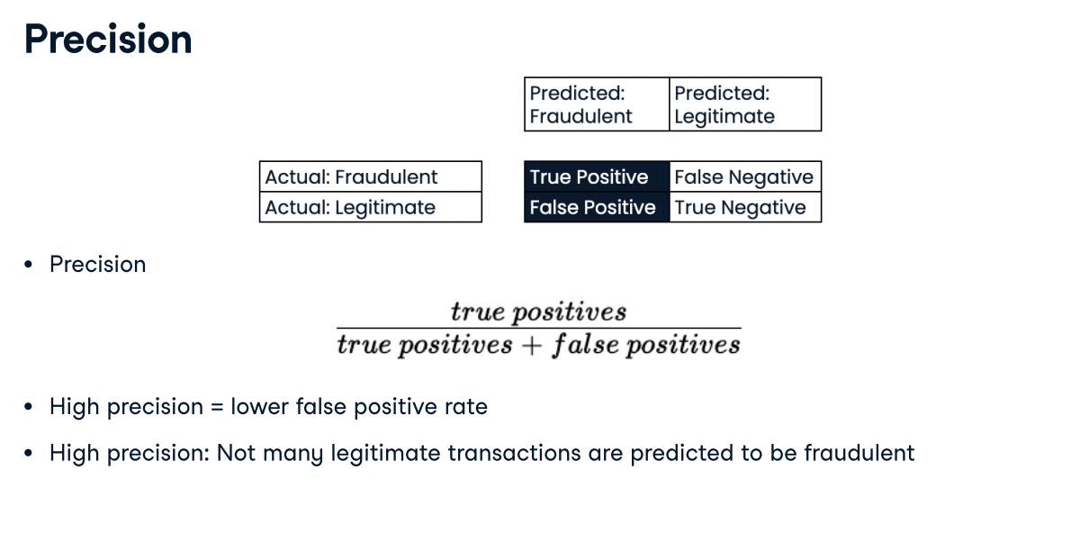
In this exercise, you will be provided with three different classification problems, and your task is to select the problem where precision is best suited as the primary metric.
Answer:A model predicting if a customer is a high-value lead for a sales team with limited capacity. With limited capacity, the sales team needs the model to return the highest proportion of true positives compared to all predicted positives, thus minimizing wasted effort.
Assessing a diabetes prediction classifier
In this chapter you'll work with the diabetes_df dataset introduced previously.
The goal is to predict whether or not each individual is likely to have diabetes based on the features body mass index (BMI) and age (in years). Therefore, it is a binary classification problem. A target value of 0 indicates that the individual does not have diabetes, while a value of 1 indicates that the individual does have diabetes.
diabetes_df has been preloaded for you as a pandas DataFrame and split into X_train, X_test, y_train, and y_test. In addition, a KNeighborsClassifier() has been instantiated and assigned to knn.
You will fit the model, make predictions on the test set, then produce a confusion matrix and classification report.
Instructions:
- Import confusion_matrix and classification_report.
- Fit the model to the training data.
- Predict the labels of the test set, storing the results as y_pred.
- Compute and print the confusion matrix and classification report for the test labels versus the predicted labels.
df = pd.read_csv('./datasets/diabetes_clean.csv', index_col=None)
display(df.head())

# diabetes_df = df.loc[(df['glucose'] != 0) & (df['bmi'] != 0)].copy()
diabetes_df = df.copy()

X = diabetes_df[["bmi", "age"]].values
y = diabetes_df["diabetes"].values

X_train, X_test, y_train, y_test = train_test_split(X, y, test_size=0.3, random_state=42)
print(X_train.shape, y_train.shape)
from sklearn.metrics import classification_report, confusion_matrix

knn = KNeighborsClassifier(n_neighbors=6)

# Fit the model to the training data
knn.fit(X_train, y_train)

# Predict the labels of the test data: y_pred
y_pred = knn.predict(X_test)

# Generate the confusion matrix and classification report
print(confusion_matrix(y_test, y_pred))
print(classification_report(y_test, y_pred))
The model produced 116 true positives, 33 true negatives, 35 false negatives, and 47 false positives. The classification report shows a better F1-score for the zero class, which represents individuals who do not have diabetes.
X = churn_df.copy().drop(['churn'], axis=1).values
y = churn_df["churn"].values
from sklearn.linear_model import LogisticRegression

logreg = LogisticRegression(max_iter=10000)
X_train, X_test, y_train, y_test = train_test_split(X, y, test_size=0.3, random_state=42)

logreg.fit(X_train, y_train)
y_pred = logreg.predict(X_test)

# Predicting probabilities
y_pred_probs = logreg.predict_proba(X_test)[:, 1]
print(y_pred_probs[0])
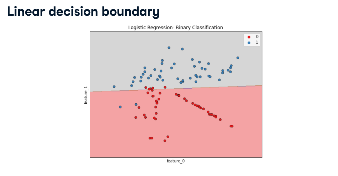
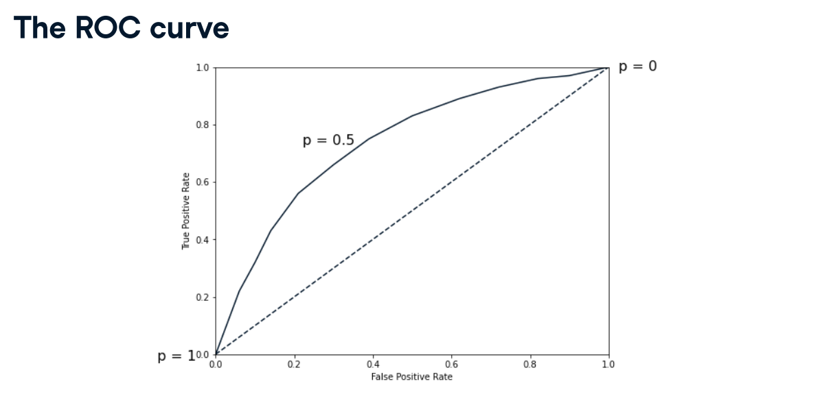
Probability thresholds
- By default, logistic regression threshold = 0.5
- Not speci,c to logistic regression
- KNN classi,ers also have thresholds
- What happens if we vary the threshold?
ROC curve
import matplotlib.pyplot as plt
from sklearn.metrics import roc_curve

fpr, tpr, thresholds = roc_curve(y_test, y_pred_probs)
plt.plot([0, 1], [0, 1], 'k--')
plt.plot(fpr, tpr)
plt.xlabel('False Positive Rate')
plt.ylabel('True Positive Rate')
plt.title('Logistic Regression ROC Curve')
plt.show()
from sklearn.metrics import roc_auc_score
print(roc_auc_score(y_test, y_pred_probs))
pretty good, AUC is 82%.
Building a logistic regression model
In this exercise, you will build a logistic regression model using all features in the diabetes_df dataset. The model will be used to predict the probability of individuals in the test set having a diabetes diagnosis.
The diabetes_df dataset has been split into X_train, X_test, y_train, and y_test, and preloaded for you.
Instructions:
- Import LogisticRegression.
- Instantiate a logistic regression model, logreg.
- Fit the model to the training data.
- Predict the probabilities of each individual in the test set having a diabetes diagnosis, storing the array of positive probabilities as y_pred_probs.
X = diabetes_df.drop(['diabetes'], axis=1).values
y = diabetes_df["diabetes"].values

X_train, X_test, y_train, y_test = train_test_split(X, y, test_size=0.3, random_state=42)
print(X_train.shape, y_train.shape)
from sklearn.linear_model import LogisticRegression

# Instantiate the model
logreg = LogisticRegression( max_iter=10000)

# Fit the model
logreg.fit(X_train, y_train)

# Predict probabilities
y_pred_probs = logreg.predict_proba(X_test)[:, 1]
y_pred = logreg.predict(X_test)

print(sorted(y_pred_probs[:10]))
Nicely done! Notice how the probability of a diabetes diagnosis for the first 10 individuals in the test set ranges from 0.01 to 0.79. Now let's plot the ROC curve to visualize performance using different thresholds.
The ROC curve
Now you have built a logistic regression model for predicting diabetes status, you can plot the ROC curve to visualize how the true positive rate and false positive rate vary as the decision threshold changes.
The test labels, y_test, and the predicted probabilities of the test features belonging to the positive class, y_pred_probs, have been preloaded for you, along with matplotlib.pyplot as plt.
You will create a ROC curve and then interpret the results.
Instructions:
- Import roc_curve.
- Calculate the ROC curve values, using y_test and y_pred_probs, and unpacking the results into fpr, tpr, and thresholds.
- Plot true positive rate against false positive rate.
print(roc_auc_score(y_test, y_pred_probs))
from sklearn.metrics import roc_curve

# Generate ROC curve values: fpr, tpr, thresholds
fpr, tpr, thresholds = roc_curve(y_test, y_pred_probs)

plt.plot([0, 1], [0, 1], 'k--')

# Plot tpr against fpr
plt.plot(fpr, tpr)
plt.xlabel('False Positive Rate')
plt.ylabel('True Positive Rate')
plt.title('ROC Curve for Diabetes Prediction')
plt.show()
Question: Well done on producing the ROC curve for the diabetes prediction model. But, what does the plot tell you about the model's performance?
Possible Answers:
The model is about as good as randomly guessing the class of each observation.
The model is much worse than randomly guessing the class of each observation.
The model is much better than randomly guessing the class of each observation.
It is not possible to conclude whether the model performs better or worse than randomly guessing the class of each observation.
Ans:The model is much better than randomly guessing the class of each observation. The ROC curve is above the dotted line, so the model performs better than randomly guessing the class of each observation. (AUC value is 0.796523178807947, which is pretty good)
ROC AUC
The ROC curve you plotted in the last exercise looked promising.
Now you will compute the area under the ROC curve, along with the other classification metrics you have used previously.
The confusion_matrix and classification_report functions have been preloaded for you, along with the logreg model you previously built, plus X_train, X_test, y_train, y_test. Also, the model's predicted test set labels are stored as y_pred, and probabilities of test set observations belonging to the positive class stored as y_pred_probs.
A knn model has also been created and the performance metrics printed in the console, so you can compare the roc_auc_score, confusion_matrix, and classification_report between the two models.
Instructions:
- Import roc_auc_score.
- Calculate and print the ROC AUC score, passing the test labels and the predicted positive class probabilities.
- Calculate and print the confusion matrix.
- Call classification_report().
from sklearn.metrics import roc_auc_score

# Calculate roc_auc_score
print(roc_auc_score(y_test, y_pred_probs))

# Calculate the confusion matrix
print(confusion_matrix(y_test, y_pred))

# Calculate the classification report
print(classification_report(y_test, y_pred))
Did you notice that logistic regression performs better than the KNN model across all the metrics you calculated? A ROC AUC score of 0.7965 means this model is 60% better than a chance model at correctly predicting labels! scikit-learn makes it easy to produce several classification metrics with only a few lines of code.
Hyperparameter tuning
Hyperparameter tuning
- Ridge/lasso regression: Choosing
alpha - KNN: Choosing
n_neighbors - Hyperparameters: Parameters we specify before fitting the model
- Like alpha and
n_neighbors
- Like alpha and
Choosing the correct hyperparameters:
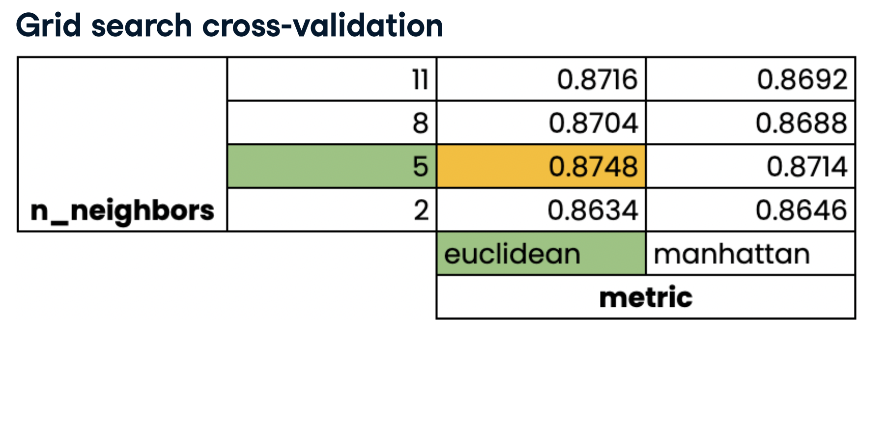
- Try lots of di(erent hyperparameter values
- Fit all of them separately
- See how well they perform
- Choose the best performing values
- This is called hyperparameter tuning
- It is essential to use cross-validation to avoid over,2ing to the test set
- We can still split the data and perform cross-validation on the training set
- We withhold the test set for ,nal evaluation
sales_df = pd.read_csv('./datasets/advertising_and_sales_clean.csv', index_col=None)
display(sales_df.head())


# Create X from the radio column's values (.values to make sure they are numpy array)
X = sales_df[['radio','social_media']].values

# Create y from the sales column's values
y = sales_df['sales'].values

X_train, X_test, y_train, y_test = train_test_split(X, y, test_size=0.3, random_state=42)
from sklearn.linear_model import Ridge
from sklearn.model_selection import GridSearchCV, KFold

kf = KFold(n_splits=5, shuffle=True, random_state=42)
param_grid = {  "alpha": np.arange(0.0001, 1, 10),
                "solver": ["sag", "lsqr"]}

ridge = Ridge()
ridge_cv = GridSearchCV(ridge, param_grid, cv=kf)
ridge_cv.fit(X_train, y_train)
print(ridge_cv.best_params_, ridge_cv.best_score_)
test_score = ridge_cv.score(X_test, y_test)
print(test_score)
Limitations of GridSearchCV:
- 3-fold cross-validation, 1 hyperparameter, 10 total values = 30 ,ts
- 10 fold cross-validation, 3 hyperparameters, 30 total values = 900 ,ts
An alternative approach RandomizedSearchCV
from sklearn.model_selection import RandomizedSearchCV
kf = KFold(n_splits=5, shuffle=True, random_state=42)
param_grid = {'alpha': np.arange(0.0001, 1, 10),
"solver": ['sag', 'lsqr']}
ridge = Ridge()
ridge_cv = RandomizedSearchCV(ridge, param_grid, cv=kf, n_iter=2)
ridge_cv.fit(X_train, y_train)
print(ridge_cv.best_params_, ridge_cv.best_score_)
test_score = ridge_cv.score(X_test, y_test)
print(test_score)
Hyperparameter tuning with GridSearchCV
Now you have seen how to perform grid search hyperparameter tuning, you are going to build a lasso regression model with optimal hyperparameters to predict blood glucose levels using the features in the diabetes_df dataset.
X_train, X_test, y_train, and y_test have been preloaded for you. A KFold() object has been created and stored for you as kf, along with a lasso regression model as lasso.
Instructions:
- Import GridSearchCV.
- Set up a parameter grid for "alpha", using np.linspace() to create 20 evenly spaced values ranging from 0.00001 to 1.
- Call GridSearchCV(), passing lasso, the parameter grid, and setting cv equal to kf.
- Fit the grid search object to the training data to perform a cross-validated grid search.
X = diabetes_df.drop(["glucose"], axis=1).values
y = diabetes_df["glucose"].values

X_train, X_test, y_train, y_test = train_test_split(X, y, test_size=0.2, random_state=42)
print(X_train.shape, y_train.shape)
from sklearn.model_selection import GridSearchCV, KFold
from sklearn.linear_model import Lasso


kf = KFold(n_splits=5, shuffle=True, random_state=42)

# Set up the parameter grid
param_grid = {"alpha": np.linspace(0.00001, 1, 20)}

# Instantiate lasso_cv
lasso = Lasso()
lasso_cv = GridSearchCV(lasso, param_grid, cv=kf)

# Fit to the training data
lasso_cv.fit(X_train, y_train)
print("Tuned lasso paramaters: {}".format(lasso_cv.best_params_))
print("Tuned lasso score: {}".format(lasso_cv.best_score_))
Unfortunately, the best model only has an R-squared score of 0.33, highlighting that using the optimal hyperparameters does not guarantee a high performing model!
Hyperparameter tuning with RandomizedSearchCV
As you saw, GridSearchCV can be computationally expensive, especially if you are searching over a large hyperparameter space. In this case, you can use RandomizedSearchCV, which tests a fixed number of hyperparameter settings from specified probability distributions.
Training and test sets from diabetes_df have been pre-loaded for you as X_train. X_test, y_train, and y_test, where the target is "diabetes". A logistic regression model has been created and stored as logreg, as well as a KFold variable stored as kf.
You will define a range of hyperparameters and use RandomizedSearchCV, which has been imported from sklearn.model_selection, to look for optimal hyperparameters from these options.
Instructions:
- Create params, adding "l1" and "l2" as penalty values, setting C to a range of 50 float values between 0.1 and 1.0, and class_weight to either "balanced" or a dictionary containing 0:0.8, 1:0.2.
- Create the Randomized Search CV object, passing the model and the parameters, and setting cv equal to kf.
- Fit logreg_cv to the training data.
- Print the model's best parameters and accuracy score.
X = diabetes_df.drop(["diabetes"], axis=1).values
y = diabetes_df["diabetes"].values

X_train, X_test, y_train, y_test = train_test_split(X, y, test_size=0.2, random_state=42)
print(X_train.shape, y_train.shape)
from sklearn.model_selection import RandomizedSearchCV
# Create the parameter space
params = {"penalty": ["l1", "l2"],
         "tol": np.linspace(0.0001, 1.0, 50),
         "C": np.linspace(0.1, 1, 50),
         "class_weight": ["balanced", {0:0.8, 1:0.2}]}

log_reg = LogisticRegression(solver='liblinear',max_iter=10000)
# Instantiate the RandomizedSearchCV object
logreg_cv = RandomizedSearchCV(log_reg, params, cv=kf)

# Fit the data to the model
logreg_cv.fit(X_train, y_train)

# Print the tuned parameters and score
print("Tuned Logistic Regression Parameters: {}".format(logreg_cv.best_params_))
print("Tuned Logistic Regression Best Accuracy Score: {}".format(logreg_cv.best_score_))
Even without exhaustively trying every combination of hyperparameters, the model has an accuracy of over 70% on the test set! So far we have worked with clean datasets; however, in the next chapter, we will discuss the steps required to transform messy data before building supervised learning models.
